Example 1 - Square Ice Shelf
This notebook provides a simple example of computing steady-state ice velocity in a square ice shelf. The primary steps include:
Define the model mesh based on a specified domain outline and resolution.
Define the model mask to assign regions of ice/no-ice and grounded/floating ice.
Parameterize the model to assign required geometry and initialization fields
Define boundary conditions around the model extent.
Define the flow approximation to use
Execute the model
Visualise the model results
import os
import pyissm
import numpy as np
from pathlib import Path
import matplotlib.pyplot as plt
Setup your modelling environment
This notebook is designed to be executed on the NCI Gadi supercomputer, or locally on your personal machine. The notebook assumes the location of additional required assests and model execution directories that may be affected by read/write permissions on NCI Gadi, as well as the installation location of pyISSM. Below, we provide information on necessary filesystem requirements to execute this notebook.
NCI Gadi Supercomputer
By default, we assume that users have installed pyISSM (and therefore, this notebook) in their home directory: /home/<group>/<user>/pyISSM/. We refer to this path as pyissm_home.
Local machine
By default, we assume that users have installed pyISSM (and therefore, this notebook) in their home directory: ~/pyISSM/. We refer to this path as pyissm_home
Required paths
To ensure successful execution of this notebook, users must ensure the following paths are defined correctly in the below cell:
tutorial_dir = <PATH_TO_NOTEBOOK>where this notebook is located. By default, this is assumed to bepyissm_home/tutorialstutorial_asset_dir = <PATH_TO_ASSETS>where all tutorials assets are located. By default, this is assumed to bepyissm_home/tutorials/assetsexecution_dir = <PATH_TO_DIRECTORY>where model files will be saved. You must haverwxpermissions for this directory. By default, this is assumed to bepyissm_home/tutorials/models
NOTE: execution_dir must be different from the current working directory of your Python kernel.
## Set required paths
tutorial_dir = str(Path.home() / 'pyISSM' / 'tutorials')
asset_dir = tutorial_dir + '/assets'
execution_dir = tutorial_dir + '/models'

# Check that execution directory exists. If not, create it
if not os.path.isdir(execution_dir):
    os.mkdir(execution_dir)

# Print the paths for visibility
print(f"The following `tutorial_dir` is set: {tutorial_dir}")
print(f"The following `asset_dir` is set: {asset_dir}")
print(f"The following `execution_dir` is set: {execution_dir}")
The following `tutorial_dir` is set: /home/565/lb9857/pyISSM/tutorials
The following `asset_dir` is set: /home/565/lb9857/pyISSM/tutorials/assets
The following `execution_dir` is set: /home/565/lb9857/pyISSM/tutorials/models
1. Model mesh
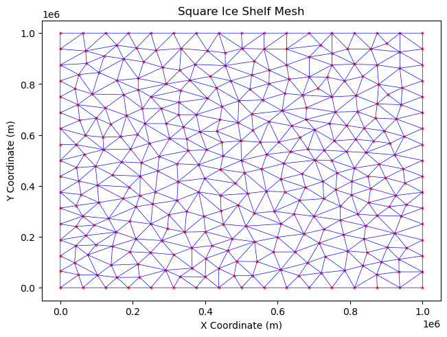
Here, we use the triangle meshing tool to build an irregular mesh with a resolution of 50 km. After the model mesh is built, all mesh information is stored in the md.mesh model sub-class. We can view the model mesh information by simply inspecting md.mesh. Below, we can see that the generated mesh has 614 elements (md.mesh.numberofelements) and 340 vertices (md.mesh.numberofvertices).
We can also visualise the mesh using pyissm.plot.plot_mesh2d().
# Create an empty model
md = pyissm.model.Model()

md
   ISSM Model Class

               mesh:  mesh properties
               mask:  defines grounded and floating elements
           geometry:  surface elevation, bedrock topography, ice thickness, ...
          constants:  physical constants
                smb:  surface mass balance
      basalforcings:  bed forcings
          materials:  material properties
             damage:  damage propagation laws
           friction:  basal friction / drag properties
       flowequation:  flow equations
       timestepping:  timestepping for transient models
     initialization:  initial guess / state
              rifts:  rifts properties
         solidearth:  solidearth inputs and settings
                dsl:  dynamic sea level
              debug:  debugging tools (valgrind, gprof
            verbose:  verbosity level in solve
           settings:  settings properties
           toolkits:  PETSc options for each solution
            cluster:  cluster parameters (number of CPUs...)
   balancethickness:  parameters for balancethickness solution
      stressbalance:  parameters for stressbalance solution
      groundingline:  parameters for groundingline solution
          hydrology:  parameters for hydrology solution
      masstransport:  parameters for masstransport solution
            thermal:  parameters for thermal solution
        steadystate:  parameters for steadystate solution
          transient:  parameters for transient solution
           levelset:  parameters for moving boundaries (level-set method)
            calving:  parameters for calving
    frontalforcings:  parameters for frontalforcings
                esa:  parameters for elastic adjustment solution
           sampling:  parameters for stochastic sampler
               love:  parameters for love solution
           autodiff:  automatic differentiation parameters
          inversion:  parameters for inverse methods
                qmu:  Dakota properties
                amr:  adaptive mesh refinement properties
   outputdefinition:  output definition
            results:  model results
       radaroverlay:  radar image for plot overlay
      miscellaneous:  miscellaneous fields
  stochasticforcing:  stochasticity applied to model forcings
# Build a model mesh using the domain outline (SquareShelf_DomainOutline.exp) with a resolution of 50 km.
md = pyissm.model.mesh.triangle(md,
                                domain_name = asset_dir + '/Exp/SquareIceShelf_DomainOutline.exp',
                                resolution = 50000
                               )

# Inspect the created mesh
md.mesh
   2D tria Mesh (horizontal):
      Elements and vertices:
         numberofelements       : 614             -- number of elements
         numberofvertices       : 340             -- number of vertices
         elements               : (614, 3)        -- vertex indices of the mesh elements
         x                      : (340,)          -- vertices x coordinate [m]
         y                      : (340,)          -- vertices y coordinate [m]
         edges                  : N/A             -- edges of the 2d mesh (vertex1 vertex2 element1 element2)
         numberofedges          : 0               -- number of edges of the 2d mesh

      Properties:
         vertexonboundary       : (340,)          -- vertices on the boundary of the domain flag list
         segments               : (64, 3)         -- edges on domain boundary (vertex1 vertex2 element)
         segmentmarkers         : (64,)           -- number associated to each segment
         vertexconnectivity     : (340, 101)      -- list of elements connected to vertex_i
         elementconnectivity    : (614, 3)        -- list of elements adjacent to element_i
         average_vertex_conne...: 25              -- average number of vertices connected to one vertex

      Extracted model:
         extractedvertices      : N/A             -- vertices extracted from the model
         extractedelements      : N/A             -- elements extracted from the model

      Projection:
         lat                    : N/A             -- vertices latitude [degrees]
         long                   : N/A             -- vertices longitude [degrees]
         epsg                   : 0               -- EPSG code (ex: 3413 for UPS Greenland, 3031 for UPS Antarctica)
         scale_factor           : N/A             -- Projection correction for volume, area, etc. computation
# Plot the mesh with customised options
fig, ax = pyissm.plot.plot_mesh2d(md,
                                  color = 'blue',
                                  linewidth = 0.5,
                                  show_nodes = True,
                                  node_kwargs = {'s': 20,
                                                 'color': 'red',
                                                 'alpha': 0.5})

# We can interact with the plot using stamdard matplotlib functions
ax.set_xlabel('X Coordinate (m)')
ax.set_ylabel('Y Coordinate (m)')
ax.set_title('Square Ice Shelf Mesh')
Text(0.5, 1.0, 'Square Ice Shelf Mesh')
2. Model Mask
The md.mask.ice_levelset and md.mask.ocean_levelset fields interact to define where there is grounded ice, floating ice, ice-free regions, and open ocean within the model domain, as follows:
ice_levelset< 0: Ice presentice_levelset= 0: Ice-front positionice_levelset> 0: No ice presentocean_levelset<0: Ocean presentocean_levelset= 0: Coastline / grounding lineocean_levelset> 0: No ocean present
In this example, the entire domain is floating ice. We can use the set_mask() function to efficiently define the md.mask fields.
After the mask is defined, all mask information is stored in the md.mask model sub-class. We can view the mask information by simply inspecting md.mask. Below, we can see that the ice_levelset and ocean_levelset fields have a size of (340, 0), consistent with md.mesh.numberofvertices (i.e., these fiels are defined on the model vertices).
To ensure the mask is defined as we expect, we can visualise the ice_levelset and ocean_levelset fields. In addition, we can visualise how these fields interact within the model to confirm regions that are defined as “floating ice” in this example.
# Define the mask: all ice is floating
md = pyissm.model.param.set_mask(md,
                                 floating_ice_name = 'all',
                                 grounded_ice_name = None)

# Inspect the mask
md.mask
   mask parameters:
         ice_levelset           : (340,)          -- presence of ice if < 0, icefront position if = 0, no ice if > 0
         ocean_levelset         : (340,)          -- presence of ocean if < 0, coastline/grounding line if = 0, no ocean if > 0
# Visuale the mask
fig, (ax1, ax2, ax3) = plt.subplots(1, 3, figsize=(12, 4))

## Visualise the `ice_levelset` field
pyissm.plot.plot_model_field(md,
                             md.mask.ice_levelset,
                             show_cbar = True,
                             show_mesh = True,
                             ax = ax1)
ax1.set_title('md.mask.ice_levelset')

## Visualise the `ocean_levelset` field
pyissm.plot.plot_model_field(md,
                             md.mask.ocean_levelset,
                             show_cbar = True,
                             show_mesh = True,
                             ax = ax2)
ax2.set_title('md.mask.ocean_levelset')

## Visualise "floating ice" elements
pyissm.plot.plot_model_elements(md,
                                ice_levelset = md.mask.ice_levelset,
                                ocean_levelset = md.mask.ocean_levelset,
                                type = 'floating_ice_elements',
                                show_mesh = True,
                                ax = ax3)
ax3.set_title('Floating ice elements')

plt.tight_layout()
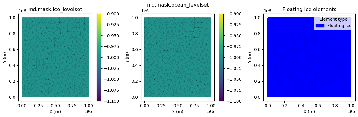
We can see that the individual mask fields (i.e. ice_levelset and ocean_levelset) both have constant values of -1. As a result, the entire model domain is considered “floating ice”. There is no grounded ice or open ocean within the model domain.
3. Parameterisation
Before we can execute a model, we must “parameterise” the model to define necessary components. This includes specifying model components such as ice geometry, initial conditions, friction representation, etc.
Warning
pyissm.model.param.parameterize()
In this example, we explicitly include the code used to parameterise the model. However, you might choose to move this parameterisation code to a secondary *.py file and use pyissm.model.param.parameterize() instead.
This functions exactly the same as running the code directly, but helps to keep your main model execution scripts clean.
Define geometry
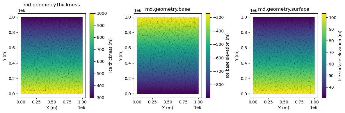
In this example, we use an idealised ice thickness that ranges from 300 to 1000 m. From this, we define an ice base (assuming hydrostatic equilibrium) and calculate an associated ice surface. All geometry information is stored in the md.geometry model sub-class. We can view the model geometry information by simply inspecting md.geometry.
We can visualise the model geometry fields using the pyissm.plot.plot_model_field() function.
# Define constants
hmin = 300
hmax = 1000
ymin = np.nanmin(md.mesh.y)
ymax = np.nanmax(md.mesh.y)

# Assign geometry to the model
md.geometry.thickness = hmax + (hmin - hmax) * (md.mesh.y - ymin) / (ymax - ymin)
md.geometry.base = - md.materials.rho_ice / md.materials.rho_water * md.geometry.thickness
md.geometry.surface = md.geometry.base + md.geometry.thickness

# Inspect the geometry
md.geometry
   geometry parameters:
         surface                : (340,)          -- ice upper surface elevation [m]
         thickness              : (340,)          -- ice thickness [m]
         base                   : (340,)          -- ice base elevation [m]
         bed                    : N/A             -- bed elevation [m]
         hydrostatic_ratio      : N/A             -- hydrostatic ratio for floating ice
# Visualise the model geometry
fig, (ax1, ax2, ax3) = plt.subplots(1, 3, figsize=(12, 4))

## Ice thickness
pyissm.plot.plot_model_field(md,
                             md.geometry.thickness,
                             show_cbar = True,
                             show_mesh = True,
                             ax = ax1,
                             cbar_kwargs = {'label': 'Ice thickness (m)'})
ax1.set_title('md.geometry.thickness')

## Ice base
pyissm.plot.plot_model_field(md,
                             md.geometry.base,
                             show_cbar = True,
                             show_mesh = True,
                             ax = ax2,
                             cbar_kwargs = {'label': 'Ice base elevation (m)'})
ax2.set_title('md.geometry.base')

## Ice surface
pyissm.plot.plot_model_field(md,
                             md.geometry.surface,
                             show_cbar = True,
                             show_mesh = True,
                             ax = ax3,
                             cbar_kwargs = {'label': 'Ice surface elevation (m)'})
ax3.set_title('md.geometry.surface')

plt.tight_layout()
Define friction
In this example, because all ice is floating, no basal friction is applied. Here, we can define a constant value of 0 to all friction fields. Note that ISSM requires that some friction fields are defined on vertices (e.g., md.friction.coefficient), while others are defined on elements (e.g., md.friction.p). The required size of each the field is checked by pyISSM before a model file is executed. All friction information is stored in the md.friction model sub-class. We can view the model friction information by simply inspecting md.geometry.
# Define friction parameters
md.friction.coefficient = np.zeros(md.mesh.numberofvertices, )
md.friction.p = np.zeros(md.mesh.numberofelements, )
md.friction.q = np.zeros(md.mesh.numberofelements, )

# Inspect friction parameters
md.friction
Basal shear stress parameters: Sigma_b = coefficient^2 * Neff ^r * |u_b|^(s - 1) * u_b,
(effective stress Neff = rho_ice * g * thickness + rho_water * g * base, r = q / p and s = 1 / p)
         coefficient            : (340,)          -- friction coefficient [SI]
         p                      : (614,)          -- p exponent
         q                      : (614,)          -- q exponent
         coupling               : 0               -- Coupling flag 0: uniform sheet (negative pressure ok, default), 1: ice pressure only, 2: water pressure assuming uniform sheet (no negative pressure), 3: use provided effective_pressure, 4: used coupled model (not implemented yet)
         linearize              : 0               -- 0: not linearized, 1: interpolated linearly, 2: constant per element (default is 0)
         effective_pressure     : N/A             -- Effective Pressure for the forcing if not coupled [Pa]
         effective_pressure_l...: 0               -- Neff do not allow to fall below a certain limit: effective_pressure_limit * rho_ice * g * thickness (default 0)
Define initial ice velocity
In this example, we define an initial velocity of 0 across the entire model domain. All initialization information is stored on the md.initialization model sub-class. We can view the model initialization information by simply inspecting md.initialization.
# Define initial velocities
md.initialization.vx = np.zeros(md.mesh.numberofvertices, )
md.initialization.vy = np.zeros(md.mesh.numberofvertices, )
md.initialization.vz = np.zeros(md.mesh.numberofvertices, )
md.initialization.vel = np.zeros(md.mesh.numberofvertices, )

# Inspect initialization fields
md.initialization
   initial field values:
         vx                     : (340,)          -- x component of velocity [m/yr]
         vy                     : (340,)          -- y component of velocity [m/yr]
         vz                     : (340,)          -- z component of velocity [m/yr]
         vel                    : (340,)          -- velocity norm [m/yr]
         pressure               : N/A             -- pressure [Pa]
         temperature            : N/A             -- temperature [K]
         enthalpy               : N/A             -- enthalpy [J]
         waterfraction          : N/A             -- fraction of water in the ice
         watercolumn            : N/A             -- thickness of subglacial water [m]
         sediment_head          : N/A             -- sediment water head of subglacial system [m]
         epl_head               : N/A             -- epl water head of subglacial system [m]
         epl_thickness          : N/A             -- thickness of the epl [m]
         hydraulic_potential    : N/A             -- Hydraulic potential (for GlaDS) [Pa]
         channelarea            : N/A             -- subglaciale water channel area (for GlaDS) [m2]
         sample                 : N/A             -- Realization of a Gaussian random field
         debris                 : N/A             -- Surface debris layer [m]
         age                    : N/A             -- Initial age [yr]
Define flow law parameters
In this example, we assume all ice is -20 °C and compute ice regidity using the pyissm.tools.materials.paterson() parameterisation. Note that ISSM requires that some materials fields are defined on vertices (e.g., md.materials.rheology_B), while others are defined on elements (e.g., md.materials.rheology_n). The required size of each the field is checked by pyISSM before a model file is executed. All materials information is stored on the md.materials model sub-class. We can view the materials information by simply inspecting md.materials.
# Define materials parameters
md.materials.rheology_B = pyissm.tools.materials.paterson(273.15 - 20) * np.ones(md.mesh.numberofvertices, )
md.materials.rheology_n = 3 * np.ones(md.mesh.numberofelements, )

# Inspect the materials parameters
md.materials
   Materials (ice):
         rho_ice                : 917.0           -- ice density [kg/m^3]
         rho_water              : 1023.0          -- ocean water density [kg/m^3]
         rho_freshwater         : 1000.0          -- fresh water density [kg/m^3]
         mu_water               : 0.001787        -- water viscosity [N s/m^2]
         heatcapacity           : 2093.0          -- heat capacity [J/kg/K]
         thermalconductivity    : 2.4             -- ice thermal conductivity [W/m/K]
         temperateiceconducti...: 0.24            -- temperate ice thermal conductivity [W/m/K]
         meltingpoint           : 273.15          -- melting point of ice at 1atm in K
         latentheat             : 334000.0        -- latent heat of fusion [J/m^3]
         beta                   : 9.8e-08         -- rate of change of melting point with pressure [K/Pa]
         mixed_layer_capacity   : 3974.0          -- mixed layer capacity [W/kg/K]
         thermal_exchange_vel...: 0.0001          -- thermal exchange velocity [m/s]
         rheology_B             : (340,)          -- flow law parameter [Pa s^(1/n)]
         rheology_n             : (614,)          -- Glen's flow law exponent
         rheology_law           : 'Paterson'      -- law for the temperature dependance of the rheology: 'None', 'BuddJacka', 'Cuffey', 'CuffeyTemperate', 'Paterson', 'Arrhenius', 'LliboutryDuval', 'NyeCO2', or 'NyeH2O'
4. Boundary conditions
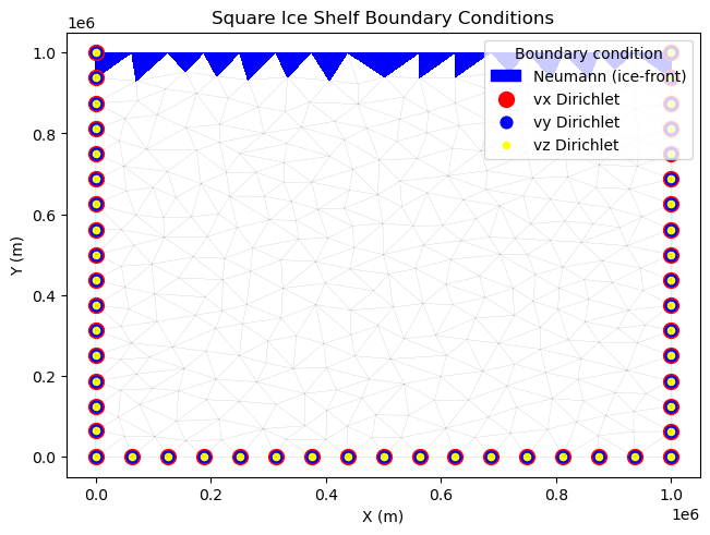
In this example, we run a “Stress balance” solution to compute ice velocity in steady-state. When running a Stress Balance solution, ISSM assumes a stress-free boundary condition at the ice sheet surface and applies a viscous friction law at the base of the ice sheet. Water pressure is applied at the ice/water interface.
As a result, we define Neumann boundary conditions along the ice-front and Dirichlet boundary conditions on all inflow nodes. Stress balance boundary conditions are defined by combination of fields in md.stressbalance.spcvx, md.stressbalance.spxvy and md.stressbalance.spcvz. We can set these automatically using pyissm.model.bc.set_ice_shelf_bc() and providing an ARGUS *.exp file that defines the ice front position. Here, since no observed velocities have been added to the model, all stress balance model boundary conditions are set to 0. All stressbalance information is stored on the md.stressbalance model sub-class. We can view the stressbalance information by simply inspecting md.stressbalance.
We can visualse the model boundary conditions using pyissm.plot.plot_model_bc(md).
# Set ice shelf boundary conditions.
md = pyissm.model.bc.set_ice_shelf_bc(md, asset_dir + '/Exp/SquareIceShelf_IceFront.exp')

# Inspect boundary conditions
# Stress balance boundary conditions are defined by combination of fields in md.stressbalance.spcvx, md.stressbalance.spcvy, md.stressbalance.spcvz.
md.stressbalance
/home/565/lb9857/gitRepos/pyISSM/src/pyissm/model/bc.py:102: UserWarning: pyissm.model.bc._set_sb_dirichlet_bc: No observed velocities found. Setting stressbalance model boundary conditions as 0.
  warnings.warn('pyissm.model.bc._set_sb_dirichlet_bc: No observed velocities found. Setting stressbalance model boundary conditions as 0.')
/home/565/lb9857/gitRepos/pyISSM/src/pyissm/model/classes/smb.py:114: UserWarning: pyissm.model.classes.smb.default: smb.mass_balance not specified -- set to 0.
  warnings.warn('pyissm.model.classes.smb.default: smb.mass_balance not specified -- set to 0.')
/home/565/lb9857/gitRepos/pyISSM/src/pyissm/model/classes/basalforcings.py:116: UserWarning: pyissm.model.classes.basalforcings.default: no groundedice_melting_rate specified -- values set as 0
  warnings.warn('pyissm.model.classes.basalforcings.default: no groundedice_melting_rate specified -- values set as 0')
/home/565/lb9857/gitRepos/pyISSM/src/pyissm/model/classes/basalforcings.py:120: UserWarning: pyissm.model.classes.basalforcings.default: no floatingice_melting_rate specified -- values set as 0
  warnings.warn('pyissm.model.classes.basalforcings.default: no floatingice_melting_rate specified -- values set as 0')
/home/565/lb9857/gitRepos/pyISSM/src/pyissm/model/bc.py:146: UserWarning: pyissm.model.bc.set_ice_shelf_bc: no balancethickness.thickening_rate specified -- values set as 0.
  warnings.warn('pyissm.model.bc.set_ice_shelf_bc: no balancethickness.thickening_rate specified -- values set as 0.')
/home/565/lb9857/gitRepos/pyISSM/src/pyissm/model/bc.py:166: UserWarning: pyissm.model.bc.set_ice_shelf_bc: No observed temperature found. No thermal boundary conditions created.
  warnings.warn('pyissm.model.bc.set_ice_shelf_bc: No observed temperature found. No thermal boundary conditions created.')
   StressBalance solution parameters:
      Convergence criteria:
         restol                 : 0.0001          -- mechanical equilibrium residual convergence criterion
         reltol                 : 0.01            -- velocity relative convergence criterion, NaN: not applied
         abstol                 : 10              -- velocity absolute convergence criterion, NaN: not applied
         isnewton               : 0               -- 0: Picard's fixed point, 1: Newton's method, 2: hybrid
         maxiter                : 100             -- maximum number of nonlinear iterations

      boundary conditions:
         spcvx                  : (340,)          -- x-axis velocity constraint (NaN means no constraint) [m / yr]
         spcvy                  : (340,)          -- y-axis velocity constraint (NaN means no constraint) [m / yr]
         spcvz                  : (340,)          -- z-axis velocity constraint (NaN means no constraint) [m / yr]

      MOLHO boundary conditions:
         spcvx_base             : N/A             -- x-axis basal velocity constraint (NaN means no constraint) [m / yr]
         spcvy_base             : N/A             -- y-axis basal velocity constraint (NaN means no constraint) [m / yr]
         spcvx_shear            : N/A             -- x-axis shear velocity constraint (NaN means no constraint) [m / yr]
         spcvy_shear            : N/A             -- y-axis shear velocity constraint (NaN means no constraint) [m / yr]

      Rift options:
         rift_penalty_threshold : 0               -- threshold for instability of mechanical constraints
         rift_penalty_lock      : 10              -- number of iterations before rift penalties are locked

      Penalty options:
         penalty_factor         : 3               -- offset used by penalties: penalty = Kmax * 10^offset
         vertex_pairing         : N/A             -- pairs of vertices that are penalized

      Hydrology layer:
         ishydrologylayer       : 0               -- (SSA only) 0: no subglacial hydrology layer in driving stress, 1: hydrology layer in driving stress

      Other:
         shelf_dampening        : 0               -- use dampening for floating ice ? Only for FS model
         FSreconditioning       : 10000000000000  -- multiplier for incompressibility equation. Only for FS model
         referential            : (340, 6)        -- local referential
         loadingforce           : (340, 3)        -- loading force applied on each point [N/m^3]
         requested_outputs      : ['default',]    -- additional outputs requested
# Visualise boundary conditions
fig, ax = pyissm.plot.plot_model_bc(md)

ax.set_title('Square Ice Shelf Boundary Conditions')
Text(0.5, 1.0, 'Square Ice Shelf Boundary Conditions')
5. Set the flow equation
This example uses the Shelfy-Stream Approximation (SSA) of the Full-Stokes equation across the whole domain. To define this, we can use pyissm.model.param.set_flow_equation(). All flow equation information is stored on the md.flowequation model sub-class. We can view the flowequation information by simply inspecting md.flowequation.
# Use the SSA flow approximation across the whole domain
md = pyissm.model.param.set_flow_equation(md, SSA = 'all')
md.flowequation
   flow equation parameters:
         isSIA                  : 0               -- is the Shallow Ice Approximation (SIA) used?
         isSSA                  : 1               -- is the Shelfy-Stream Approximation (SSA) used?
         isL1L2                 : 0               -- are L1L2 equations used?
         isMOLHO                : 0               -- are MOno-layer Higher-Order (MOLHO) equations used?
         isHO                   : 0               -- is the Higher-Order (HO) approximation used?
         isFS                   : 0               -- are the Full-FS (FS) equations used?
         isNitscheBC            : 0               -- is weakly imposed condition used?
         FSNitscheGamma         : 1000000.0       -- Gamma value for the Nitsche term (default: 1e6)
         fe_SSA                 : 'P1'            -- Finite Element for SSA: 'P1', 'P1bubble' 'P1bubblecondensed' 'P2'
         fe_HO                  : 'P1'            -- Finite Element for HO:  'P1', 'P1bubble', 'P1bubblecondensed', 'P1xP2', 'P2xP1', 'P2', 'P2bubble', 'P1xP3', 'P2xP4'
         fe_FS                  : 'MINIcondensed' -- Finite Element for FS:  'P1P1' (debugging only) 'P1P1GLS' 'MINIcondensed' 'MINI' 'TaylorHood' 'LATaylorHood' 'XTaylorHood'
         vertex_equation        : (340,)          -- flow equation for each vertex
         element_equation       : (614,)          -- flow equation for each element
         borderSSA              : (340,)          -- vertices on SSA's border (for tiling)
         borderHO               : (340,)          -- vertices on HO's border (for tiling)
         borderFS               : (340,)          -- vertices on FS' border (for tiling)
6. Execute the model
To compute the velocity of the ice shelf, we use the “Stress Balance” solution. To run this example, we use the default md.cluster as this model is small enough to run on typical HPC login nodes, or directly on local machines.
Here, the results are loaded back onto md.results once the model run has finished.
md.cluster.executionpath = execution_dir
md.miscellaneous.name = 'SquareIceShelf'
md = pyissm.model.execute.solve(md, 'Stressbalance')
Checking model consistency...
Marshalling for SquareIceShelf.bin
/home/565/lb9857/gitRepos/pyISSM/src/pyissm/model/classes/qmu.py:95: UserWarning: pyissm.model.classes.qmu::qmu not yet implemented. Turning off qmu.
  warnings.warn('pyissm.model.classes.qmu::qmu not yet implemented. Turning off qmu.')
Uploading files to cluster...
Transferring SquareIceShelf-02-23-2026-11-42-21-770209.tar.gz to cluster gadi-cpu-bdw-0240.gadi.nci.org.au...
Launching job SquareIceShelf on cluster gadi-cpu-bdw-0240.gadi.nci.org.au...

Ice-sheet and Sea-level System Model (ISSM) version  4.24
(GitHub: https://issmteam.github.io/ISSM-Documentation/ Documentation: https://github.com/ISSMteam/ISSM/)

call computational core:
   computing new velocity
write lock file:

   FemModel initialization elapsed time:   0.0227055
   Total Core solution elapsed time:       0.231375
   Linear solver elapsed time:             0.0670765 (29%)

   Total elapsed time: 0 hrs 0 min 0 sec
Waiting for job to complete...
wait_on_lock not implemented yet
Job completed -- loading results from cluster...
Retrieving results from cluster gadi-cpu-bdw-0240.gadi.nci.org.au...
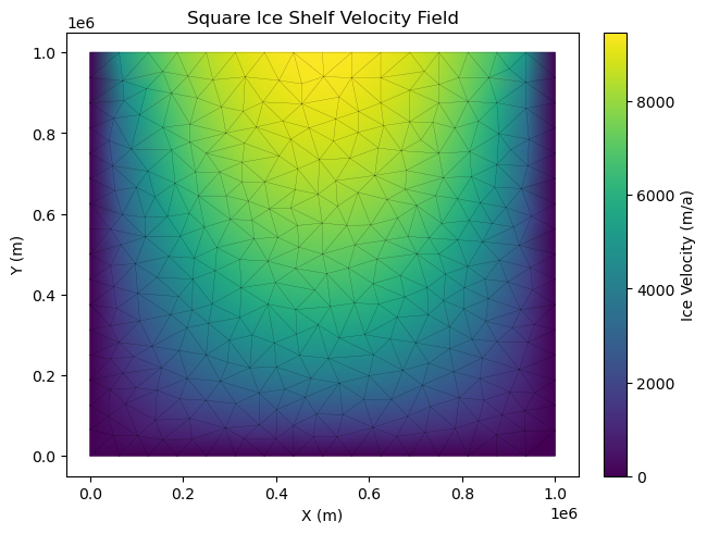
7. Visualise model results
Once the model has finised executing, results are automatically loaded to md.results. We can view the model results by inspecting md.results.StressbalanceSolution. We can see that md.results.StressbalanceSolution contains 2D fields for Vx, Vy, Vel, and Pressure. The steps and time fields are both 0 since this was not a transient simulation.
To provide a summary of the solution, including all fields, and their associated data type and shape, we can use pyissm.tools.general.summarize_solution().
We can visualise the computed ice velocity field using pyissm.model.plot_model_field().
# View a summary of the model solution
pyissm.tools.general.summarize_solution(md.results.StressbalanceSolution)
Field                               Type                 Shape / Length
---------------------------------------------------------------------------
StressbalanceConvergenceNumSteps    ndarray              (1,)
step                                int32                scalar
time                                float64              scalar
Vx                                  ndarray              (340,)
Vy                                  ndarray              (340,)
Vel                                 ndarray              (340,)
Pressure                            ndarray              (340,)
SolutionType                        str                  scalar
errlog                              list                 len=0
outlog                              str                  scalar
# Visualise the resultant velocity field
fig, ax = pyissm.plot.plot_model_field(md,
                                       field = md.results.StressbalanceSolution.Vel,
                                       show_cbar = True,
                                       cbar_kwargs={'label': 'Ice Velocity (m/a)'},
                                       show_mesh = True)
ax.set_title('Square Ice Shelf Velocity Field')
Text(0.5, 1.0, 'Square Ice Shelf Velocity Field')
8. Save model
At any stage throughout the modelling process, we can save the current model state using pyissm.model.io.save_model(). Now we’re all finished, let’s save the model next to the tutorial notebook for a rainy day!
# Save model
pyissm.model.io.save_model(md, tutorial_dir + '/ex1_SquareIceShelf.nc')