Example 2 - Pine Island Glacier
This notebook provides an example of a typical ISSM workflow to complete the following:
Build and parameterise an ISSM model
Conduct a basal friction inversion
Run a Higher-Order (HO) Stress balance simulation
We use the Pine Island Glacier (PIG) as our model domain and use a combination of observational and model output data sets to parameterise the model.
import os
import pyissm
import numpy as np
from pathlib import Path
import matplotlib.pyplot as plt
Setup your modelling environment
This notebook is designed to be executed on the NCI Gadi supercomputer, or locally on your personal machine. The notebook assumes the location of additional required assests and model execution directories that may be affected by read/write permissions on NCI Gadi, as well as the installation location of pyISSM. Below, we provide information on necessary filesystem requirements to execute this notebook.
NCI Gadi Supercomputer
By default, we assume that users have installed pyISSM (and therefore, this notebook) in their home directory: /home/<group>/<user>/pyISSM/. We refer to this path as pyissm_home.
Local machine
By default, we assume that users have installed pyISSM (and therefore, this notebook) in their home directory: ~/pyISSM/. We refer to this path as pyissm_home
Required paths
To ensure successful execution of this notebook, users must ensure the following paths are defined correctly in the below cell:
tutorial_dir = <PATH_TO_NOTEBOOK>where this notebook is located. By default, this is assumed to bepyissm_home/tutorialstutorial_asset_dir = <PATH_TO_ASSETS>where all tutorials assets are located. By default, this is assumed to bepyissm_home/tutorials/assetsexecution_dir = <PATH_TO_DIRECTORY>where model files will be saved. You must haverwxpermissions for this directory. By default, this is assumed to bepyissm_home/tutorials/models
NOTE: execution_dir must be different from the current working directory of your Python kernel.
## Set required paths
tutorial_dir = str(Path.home() / 'pyISSM' / 'tutorials')
asset_dir = tutorial_dir + '/assets'
execution_dir = tutorial_dir + '/models'

# Check that execution directory exists. If not, create it
if not os.path.isdir(execution_dir):
    os.mkdir(execution_dir)

# Print the paths for visibility
print(f"The following `tutorial_dir` is set: {tutorial_dir}")
print(f"The following `asset_dir` is set: {asset_dir}")
print(f"The following `execution_dir` is set: {execution_dir}")
The following `tutorial_dir` is set: /home/565/lb9857/pyISSM/tutorials
The following `asset_dir` is set: /home/565/lb9857/pyISSM/tutorials/assets
The following `execution_dir` is set: /home/565/lb9857/pyISSM/tutorials/models
Input datasets
This notebook requires various datasets be available for model parameterisation. By default, we make use of the ACCESS Community Cryosphere Datapool (CCD), available on NCI Gadi. However, if the CCD is not available (or not configured for local use) on your local machine, required datasets can be loaded using xarray. If you are not working on NCI Gadi (or have not configured the CCD for local use), please update the local paths to required datasets in the below cell.
NOTE: This step is also required in the assets_dir/pig_param.py parameter file.
try:
    ## BY DEFAULT: Load data using the CCD
    import ccdtools as dp
    print(f"All required datasets will be loaded from the ACCESS Community Cryosphere Datapool on {pyissm.tools.config.get_hostname()}.")

    # Initialise catalog
    catalog = dp.catalog.DataCatalog()

    # Load MEaSUREs velocity v2 dataset
    velocity = catalog.load_dataset('measures_insar_based_antarctica_ice_velocity_map', version = 'v2')

    # Load MEaSUREs BedMachine v3 dataset
    bm = catalog.load_dataset('measures_bedmachine_antarctica')
except:
    ## WORKING LOCALLY: Load data directly using xarray
    print(f"The ACCESS Community Cryosphere Datapool is not accessible on {pyissm.tools.config.get_hostname()}. Please update the paths to the required input datasets below.")
    import xarray as xr

    ## To load datasets locally using xarray, please update the following paths
    velocity = xr.open_dataset("<PATH_TO_MEASURES_V2_ICE_VELOCITY_DATASET>") # Data available here: https://nsidc.org/data/nsidc-0484/versions/2
    bm = xr.open_dataset("<PATH_TO_MEASURES_BEDMACHINCE_V3_DATASET>") # Data available here: https://nsidc.org/data/nsidc-0756/versions/3
All required datasets will be loaded from the ACCESS Community Cryosphere Datapool on gadi-cpu-bdw-0240.gadi.nci.org.au.
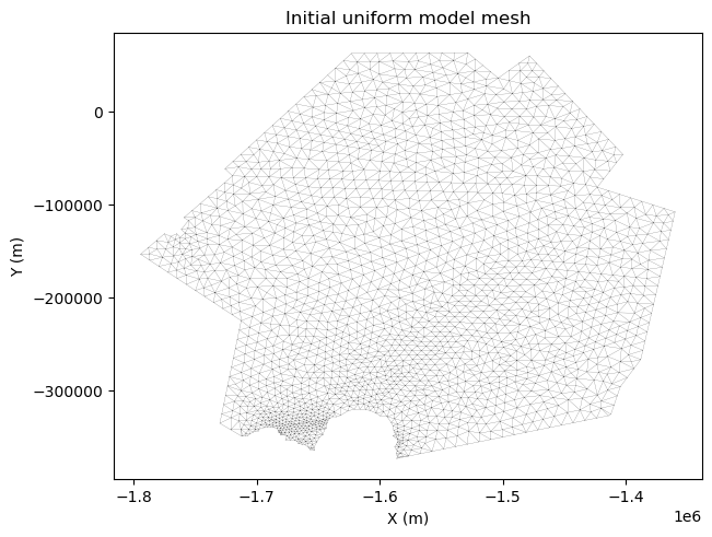
1. Model mesh
In this example, we first generate a uniform mesh with a resolution of 10 km. We then refine this mesh based on the observed velocity field using anisotropic mesh refinement. At each step, we plot the mesh and velocity field.
# Define initial mesh parameters
hinit = 10000

# Generate initial uniform mesh
md = pyissm.model.mesh.bamg(pyissm.model.Model(),
                            domain = asset_dir + '/Exp/PIG_DomainOutline.exp',
                            hmax = hinit)
# Visualise initial uniform mesh
fig, ax = pyissm.plot.plot_mesh2d(md)
ax.set_title('Initial uniform model mesh')
Text(0.5, 1.0, 'Initial uniform model mesh')
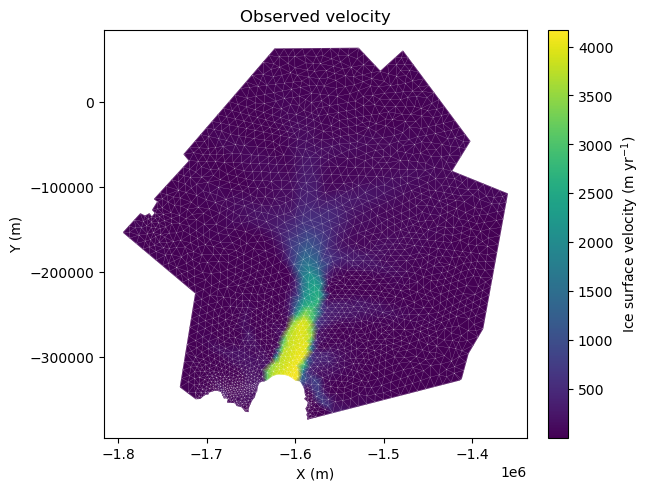
Here, we interpolate the velocity data onto the model mesh using the default “bilinear” interpolation technique. We use the fill_nan option to automatically fill remaining NaN values using nearest-neighbour (default) interpolation to ensure a complete velocity field. We then plot the observed velocity field on the model mesh, passing some optional arguments to tailor the appearance of the plot.
# Assign velocity to model
vx_mesh = pyissm.data.interp.xr_to_mesh(velocity, 'VX', md.mesh.x, md.mesh.y, fill_nan = True)
vy_mesh = pyissm.data.interp.xr_to_mesh(velocity, 'VY', md.mesh.x, md.mesh.y, fill_nan = True)
vel_mesh = np.sqrt(vx_mesh**2 + vy_mesh**2)
# Visualise velocity
fig, ax = pyissm.plot.plot_model_field(md,
                                       vel_mesh,
                                       show_mesh = True,
                                       mesh_kwargs = {'color': 'white'},
                                       show_cbar = True,
                                       cbar_kwargs = {'label': 'Ice surface velocity (m yr$^{-1}$)'})
ax.set_title('Observed velocity')
Text(0.5, 1.0, 'Observed velocity')
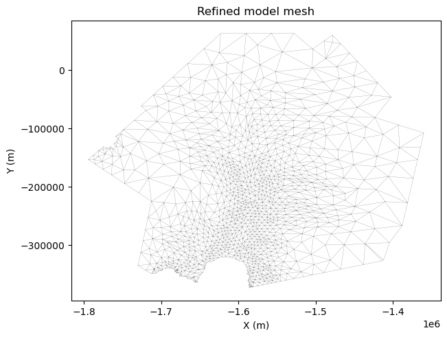
Next, we refine the model mesh based on the observed velocity field. We define a maximum (hmax) and minmum (hmin) vertex length, as well as gradation and err value for the refinement. Adjusting these parameters influences the degree of mesh refinement. We then visualise the refined mesh.
# Define mesh refinement parameters
hmax = 40000
hmin = 5000
gradation = 1.7
err = 8

# Adapt the mesh based on the velocity
md = pyissm.model.mesh.bamg(md,
                            hmax = hmax,
                            hmin = hmin,
                            gradation = gradation,
                            field = vel_mesh,
                            err = err)
# Visualise refined mesh
fig, ax = pyissm.plot.plot_mesh2d(md)
ax.set_title('Refined model mesh')
Text(0.5, 1.0, 'Refined model mesh')
Finally, we save the model mesh for use in subsequent steps. By default, this is saved alongside this notebook in the tutorial_dir.
# Save the model
pyissm.model.io.save_model(md, tutorial_dir + '/ex2_PIG_mesh.nc')
2. Model Mask
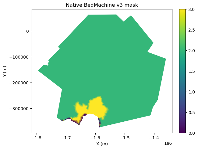
Next, we define regions of ice/no-ice and grounded/floating ice. To do this, we use the mask variable from BedMachine v3 (bm variable loaded at the beginning of this notebook). We first load the model from the precedeing step, then interpolate the mask onto the model mesh, and finally designate ice/no-ice and grounded/floating ice based on the mask values. We visualise the fields after each step.
# Load the model
md = pyissm.model.io.load_model(tutorial_dir + '/ex2_PIG_mesh.nc')
When interpolating the mask variable, we use the nearest-neighbour interpolation (`interpolation_type = ‘nearest’) to preserve the unique binary values of the mask. We then visualise the native mask on the model mesh.
# Interpolate mask to model mesh
## NOTE: Use interpolation_type = 'nearest' to retain unique values for mask
mask = pyissm.data.interp.xr_to_mesh(bm, 'mask', md.mesh.x, md.mesh.y, interpolation_type = 'nearest')
# Visuaise the mask
fig, ax = pyissm.plot.plot_model_field(md, mask, show_cbar = True)
ax.set_title('Native BedMachine v3 mask')
Text(0.5, 1.0, 'Native BedMachine v3 mask')
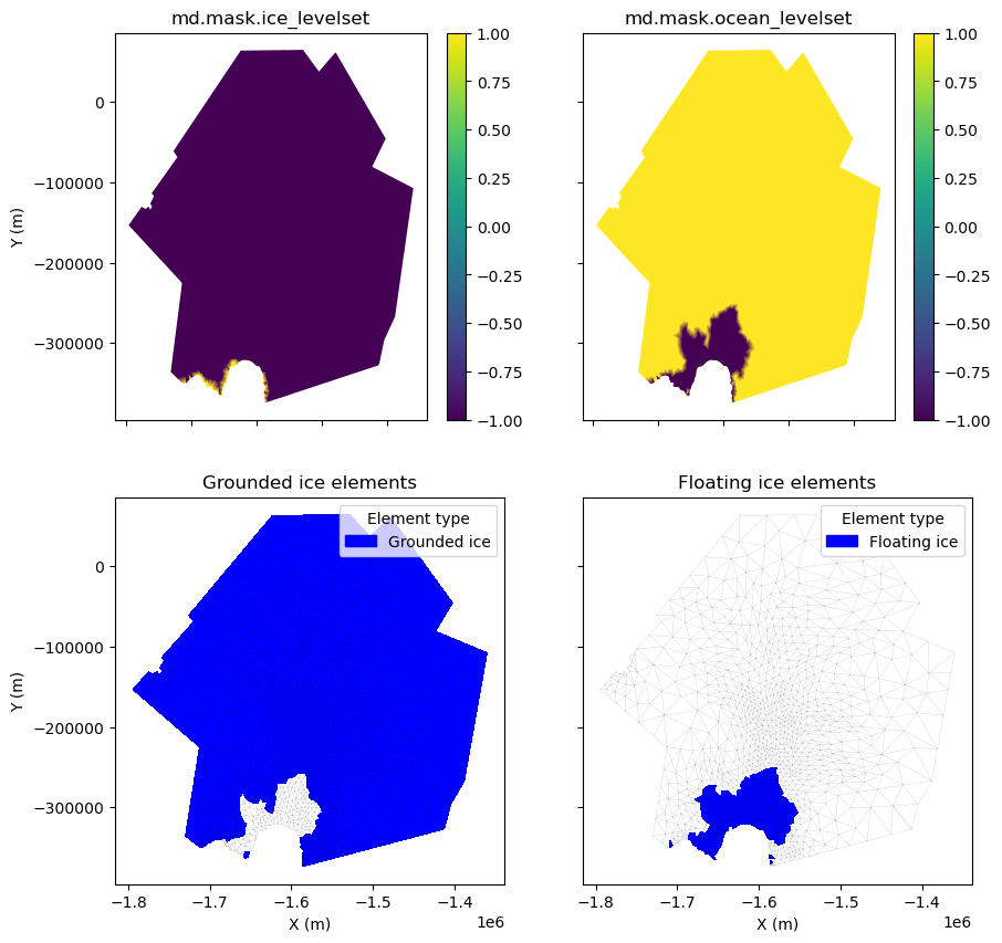
The md.mask.ice_levelset and md.mask.ocean_levelset fields interact to define where there is grounded ice, floating ice, ice-free regions, and open ocean within the model domain, as follows:
ice_levelset< 0: Ice presentice_levelset= 0: Ice-front positionice_levelset> 0: No ice presentocean_levelset<0: Ocean presentocean_levelset= 0: Coastline / grounding lineocean_levelset> 0: No ocean present
Next, we discretise the mask variable as required and visualise both the md.mask.ocean_levelset, md.mask.ice_levelset fields, as well as their interaction to define grounding ice and floating ice within the model domain. We visualise the results and save the model for future use.
# Create empty levelset variables
ice_levelset = np.full(md.mesh.numberofvertices, np.nan)
ocean_levelset = np.full(md.mesh.numberofvertices, np.nan)

# Define ice / no-ice areas
ice_levelset[mask > 0] = -1
ice_levelset[np.isnan(ice_levelset)] = 1

# Define ocean / no-ocean areas
ocean_levelset[mask == 2] = 1
ocean_levelset[mask == 3] = -1
ocean_levelset[mask == 0] = -1

# Assign to model
md.mask.ice_levelset = ice_levelset
md.mask.ocean_levelset = ocean_levelset
# Visualise elements
## NOTE: pyissm.plot.plot_model_elements() define elements as floating/grounded if ANY node of the element is considered floating/grounded. Therefore, this includes "partially floating/grounded" elements.
fig, ((ax1, ax2), (ax3, ax4)) = plt.subplots(2, 2, figsize = (10, 10), sharex = True, sharey = True)
ax1 = pyissm.plot.plot_model_field(md, md.mask.ice_levelset, ax = ax1, show_cbar = True, xlabel = '')
ax2 = pyissm.plot.plot_model_field(md, md.mask.ocean_levelset, ax = ax2, show_cbar = True, ylabel = '', xlabel = '')
ax3 = pyissm.plot.plot_model_elements(md, md.mask.ice_levelset, md.mask.ocean_levelset, type = 'grounded_ice_elements', ax = ax3)
ax4 = pyissm.plot.plot_model_elements(md, md.mask.ice_levelset, md.mask.ocean_levelset, type = 'floating_ice_elements', ax = ax4, ylabel = '')

ax1.set_title('md.mask.ice_levelset')
ax2.set_title('md.mask.ocean_levelset')
ax3.set_title('Grounded ice elements')
ax4.set_title('Floating ice elements')
Text(0.5, 1.0, 'Floating ice elements')
# Save the model
pyissm.model.io.save_model(md, tutorial_dir + '/ex2_PIG_mask.nc')
3. Parameterize Model
Before we can execute a model, we must “parameterise” the model to define necessary components. This includes specifying model components such as ice geometry, initial conditions, friction representation, etc. Here, we utilise the pyissm.model.paramparameterize() function that allows use to keep the bulk of the parameterization code separate from this execution script.
NOTE: If you are not using the ACCESS CCD to load your datsets, you’ll need to update the dataset paths at the top of the assets_dir/Param/pig_param.py file before proceeding.
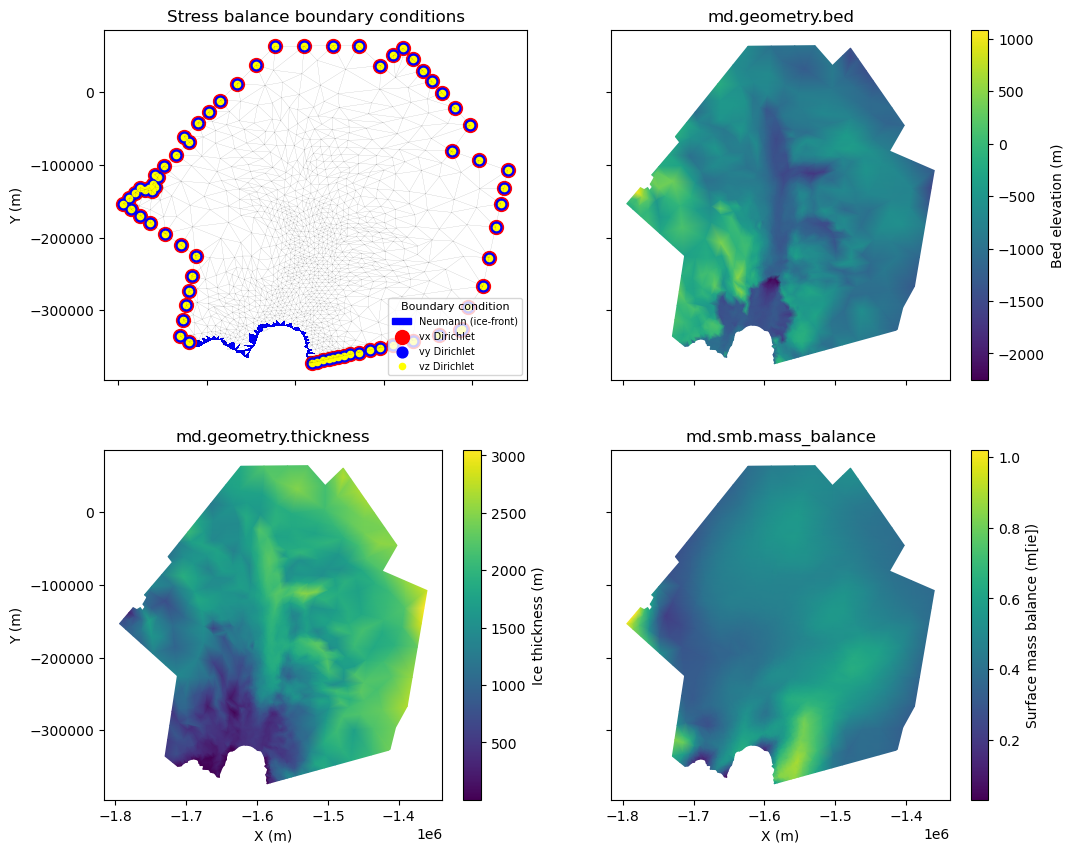
Here, we load the model from the preceding step, run the parameteriZation file, define the Shelgy-Stream Approximation (SSA) flow approximation across the whole domain, and plot some of the parameterized fields before saving the model again.
# Load the model
md = pyissm.model.io.load_model(tutorial_dir + '/ex2_PIG_mask.nc')
# Parameterize the model
md = pyissm.model.param.parameterize(md, asset_dir + '/Param/pig_param.py')
All required datasets will be loaded from the ACCESS Community Cryosphere Datapool on gadi-cpu-bdw-0240.gadi.nci.org.au.
 -- LOADING DATASETS --
/scratch/tm70/lb9857/access-cryosphere-data-pool/src/datapool/loaders.py:530: UserWarning: WARNING: Timesteps vary between various variables/files. All data files are loaded using
xr.open_mfdataset() and the timestamps are merged. As a result, all-NaN arrays are introduced
for timesteps where a given variable does not have data. Users should use caution when considering
time-varying analysis and might consider 'trimming' data to isolate all non-NaN arrays for a given variable.
  warnings.warn("WARNING: Timesteps vary between various variables/files. All data files are loaded using\n"
 -- ASSIGNING GEOMETRY --
 -- ASSIGNING INITIALIZATION FIELDS --
ll_to_xy: using south polar stereographic (Std Lat: 71S, Meridian: 0E)
 -- ASSIGNING FORCINGS --
ll_to_xy: using south polar stereographic (Std Lat: 71S, Meridian: 0E)
 -- SETTING BOUNDARY CONDITIONS --
/home/565/lb9857/gitRepos/pyISSM/src/pyissm/model/bc.py:95: UserWarning: pyissm.model.bc._set_sb_dirichlet_bc: Using observed velocities for vx and vy stressbalance model boundary conditions. vz boundary conditions are set to 0.
  warnings.warn('pyissm.model.bc._set_sb_dirichlet_bc: Using observed velocities for vx and vy stressbalance model boundary conditions. vz boundary conditions are set to 0.')
/home/565/lb9857/gitRepos/pyISSM/src/pyissm/model/classes/basalforcings.py:116: UserWarning: pyissm.model.classes.basalforcings.default: no groundedice_melting_rate specified -- values set as 0
  warnings.warn('pyissm.model.classes.basalforcings.default: no groundedice_melting_rate specified -- values set as 0')
/home/565/lb9857/gitRepos/pyISSM/src/pyissm/model/classes/basalforcings.py:120: UserWarning: pyissm.model.classes.basalforcings.default: no floatingice_melting_rate specified -- values set as 0
  warnings.warn('pyissm.model.classes.basalforcings.default: no floatingice_melting_rate specified -- values set as 0')
/home/565/lb9857/gitRepos/pyISSM/src/pyissm/model/bc.py:299: UserWarning: pyissm.model.bc.set_ice_shelf_bc: no balancethickness.thickening_rate specified -- values set as 0.
  warnings.warn('pyissm.model.bc.set_ice_shelf_bc: no balancethickness.thickening_rate specified -- values set as 0.')
# Set flow equation (SSA)
md = pyissm.model.param.set_flow_equation(md, SSA = 'all')
# Visualise various parameterized fields
fig, ((ax1, ax2), (ax3, ax4)) = plt.subplots(2, 2, figsize = (12, 10), sharex = True, sharey = True)
ax1 = pyissm.plot.plot_model_bc(md, ax = ax1, xlabel = '', legend_kwargs = {'fontsize': 7, 'title_fontsize': 8, 'loc': 'lower right'})
ax2 = pyissm.plot.plot_model_field(md, md.geometry.bed, ax = ax2, show_cbar = True, xlabel='', ylabel = '', cbar_kwargs = {'label': 'Bed elevation (m)'})
ax3 = pyissm.plot.plot_model_field(md, md.geometry.thickness, ax = ax3, show_cbar = True, cbar_kwargs = {'label': 'Ice thickness (m)'})
ax4 = pyissm.plot.plot_model_field(md, md.smb.mass_balance, ax = ax4, show_cbar = True, ylabel='', cbar_kwargs = {'label': 'Surface mass balance (m[ie])'})

ax1.set_title('Stress balance boundary conditions')
ax2.set_title('md.geometry.bed')
ax3.set_title('md.geometry.thickness')
ax4.set_title('md.smb.mass_balance')
Text(0.5, 1.0, 'md.smb.mass_balance')
# Save the model
pyissm.model.io.save_model(md, tutorial_dir + '/ex2_PIG_param.nc')
4. Perform friction inversion
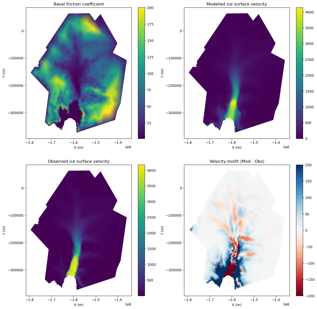
To infer the basal friction below the ice sheet, we can use inverse techniques. Here, we perform a basal friction inversion to infer the basal friction coefficient based on the default Budd friction law. All parameters that control the inversion are in md.inversion. Here, we define a minimum and maximum coefficient value of 1 and 200, respectively. We include 3 cost functions in the inversion, namely: SurfaceAbsVelMisfit (101), SurfaceLogVelMisfit (103), and DragCoefficientAbsGradient (501). We run the inversion for a maximum of 20 steps, with up to 40 iterations per step.
# Load model
md = pyissm.model.io.load_model(tutorial_dir + '/ex2_PIG_param.nc')
# Define inversion parameters
md.inversion.iscontrol = 1

md.inversion.cost_functions = [101, 103, 501]
md.inversion.cost_functions_coefficients = np.ones((md.mesh.numberofvertices, 3))
md.inversion.cost_functions_coefficients[:,0] = 50
md.inversion.cost_functions_coefficients[:,1] = 1
md.inversion.cost_functions_coefficients[:,2] = 1e-19

md.inversion.control_parameters = ['FrictionCoefficient']
md.inversion.min_parameters = 1 * np.ones(md.mesh.numberofvertices, )
md.inversion.max_parameters = 200 * np.ones(md.mesh.numberofvertices, )

md.verbose = md.verbose.deactivate_all()
md.verbose.control = 1
# Solve
md.cluster.np = 2
md.cluster.executionpath = execution_dir

md = pyissm.model.execute.solve(md, 'Stressbalance')
/home/565/lb9857/gitRepos/pyISSM/src/pyissm/model/classes/qmu.py:95: UserWarning: pyissm.model.classes.qmu::qmu not yet implemented. Turning off qmu.
  warnings.warn('pyissm.model.classes.qmu::qmu not yet implemented. Turning off qmu.')
Uploading files to cluster...
Transferring PIG-02-23-2026-11-42-38-768709.tar.gz to cluster gadi-cpu-bdw-0240.gadi.nci.org.au...
Launching job PIG on cluster gadi-cpu-bdw-0240.gadi.nci.org.au...
Ice-sheet and Sea-level System Model (ISSM) version 4.24
(GitHub: https://issmteam.github.io/ISSM-Documentation/ Documentation: https://github.com/ISSMteam/ISSM/)
call computational core:
preparing initial solution
x | Cost function f(x) | List of contributions
====================== step 1/20 ===============================
x = 0 | f(x) = 126652.7 | 117147.9 9504.79 4.143434e-16
x = 1 | f(x) = 18251.12 | 10907.76 7343.36 3.829378e-15
====================== step 2/20 ===============================
x = 0 | f(x) = 18250.18 | 10906.83 7343.348 3.829378e-15
x = 1 | f(x) = 4338.843 | 1404.739 2934.104 1.306648e-14
====================== step 3/20 ===============================
x = 0 | f(x) = 4338.655 | 1404.562 2934.093 1.306648e-14
x = 1 | f(x) = 2308.854 | 488.6028 1820.251 2.868942e-14
====================== step 4/20 ===============================
x = 0 | f(x) = 2308.742 | 488.5093 1820.233 2.868942e-14
x = 1 | f(x) = 1300.848 | 256.3423 1044.506 5.182527e-14
====================== step 5/20 ===============================
x = 0 | f(x) = 1300.814 | 256.3168 1044.497 5.182527e-14
x = 1 | f(x) = 826.75 | 191.6556 635.0944 8.694084e-14
====================== step 6/20 ===============================
x = 0 | f(x) = 826.7557 | 191.664 635.0917 8.694084e-14
x = 1 | f(x) = 802.4036 | 221.5859 580.8178 9.618449e-14
x = 0.381966 | f(x) = 755.2007 | 144.7809 610.4198 9.028355e-14
x = 0.618034 | f(x) = 766.9929 | 168.9776 598.0154 9.247507e-14
x = 0.236068 | f(x) = 760.978 | 141.9371 619.0409 8.897709e-14
x = 0.393468 | f(x) = 755.3238 | 145.5393 609.7846 9.03881e-14
x = 0.370963 | f(x) = 755.1543 | 144.112 611.0423 9.018374e-14
x = 0.369155 | f(x) = 755.1513 | 144.0039 611.1474 9.016737e-14
x = 0.365875 | f(x) = 755.1554 | 143.8225 611.3329 9.013766e-14
x = 0.368608 | f(x) = 755.1372 | 143.9534 611.1839 9.01624e-14
x = 0.367564 | f(x) = 755.153 | 143.9136 611.2394 9.015295e-14
x = 0.368382 | f(x) = 755.1391 | 143.9426 611.1965 9.016036e-14
x = 0.368817 | f(x) = 755.139 | 143.967 611.172 9.01643e-14
x = 0.368521 | f(x) = 755.1463 | 143.9593 611.1869 9.016162e-14
x = 0.368688 | f(x) = 755.1439 | 143.9658 611.1781 9.016313e-14
x = 0.368574 | f(x) = 755.1459 | 143.962 611.1839 9.01621e-14
x = 0.368641 | f(x) = 755.1447 | 143.9643 611.1804 9.016271e-14
====================== step 7/20 ===============================
x = 0 | f(x) = 755.1454 | 143.9633 611.1821 9.01624e-14
x = 1 | f(x) = 1237.653 | 795.8858 441.7673 1.22458e-13
x = 0.381966 | f(x) = 670.2858 | 137.3962 532.8896 1.021998e-13
x = 0.618034 | f(x) = 706.2768 | 213.0738 493.203 1.098949e-13
x = 0.236068 | f(x) = 690.0209 | 129.5256 560.4953 9.765374e-14
x = 0.398802 | f(x) = 669.4213 | 139.555 529.8663 1.027333e-13
x = 0.440171 | f(x) = 669.2293 | 146.6704 522.5589 1.040541e-13
x = 0.508108 | f(x) = 675.0607 | 164.1083 510.9524 1.062545e-13
x = 0.422379 | f(x) = 669.0999 | 143.4241 525.6758 1.034843e-13
x = 0.424081 | f(x) = 669.0233 | 143.644 525.3794 1.035387e-13
x = 0.430156 | f(x) = 669.0213 | 144.7096 524.3117 1.037331e-13
x = 0.433981 | f(x) = 669.0947 | 145.4541 523.6405 1.038556e-13
x = 0.427205 | f(x) = 669.1303 | 144.3051 524.8252 1.036386e-13
x = 0.431617 | f(x) = 669.0675 | 145.013 524.0545 1.037799e-13
x = 0.429029 | f(x) = 669.1315 | 144.6277 524.5038 1.03697e-13
x = 0.430714 | f(x) = 669.0673 | 144.8538 524.2135 1.037509e-13
x = 0.429726 | f(x) = 669.1034 | 144.7197 524.3837 1.037193e-13
x = 0.430369 | f(x) = 669.081 | 144.8083 524.2727 1.037399e-13
x = 0.429992 | f(x) = 669.1037 | 144.7684 524.3353 1.037278e-13
x = 0.430238 | f(x) = 669.0847 | 144.7881 524.2966 1.037357e-13
x = 0.430093 | f(x) = 669.0945 | 144.7751 524.3194 1.03731e-13
x = 0.430189 | f(x) = 669.0877 | 144.7836 524.3041 1.037341e-13
====================== step 8/20 ===============================
x = 0 | f(x) = 669.0908 | 144.7817 524.3091 1.037331e-13
x = 1 | f(x) = 684.7617 | 202.0112 482.7504 1.131169e-13
x = 0.381966 | f(x) = 631.3672 | 125.6256 505.7416 1.071276e-13
x = 0.618034 | f(x) = 647.3246 | 151.1201 496.2044 1.093428e-13
x = 0.236068 | f(x) = 630.7785 | 118.4935 512.285 1.058033e-13
x = 0.296894 | f(x) = 629.6717 | 120.1753 509.4964 1.063512e-13
x = 0.301297 | f(x) = 629.6721 | 120.376 509.2961 1.063911e-13
x = 0.298907 | f(x) = 629.6798 | 120.2806 509.3993 1.063695e-13
x = 0.27366 | f(x) = 629.83 | 119.2859 510.544 1.061412e-13
x = 0.288019 | f(x) = 629.6944 | 119.7972 509.8971 1.062709e-13
x = 0.293504 | f(x) = 629.6725 | 120.0242 509.6483 1.063205e-13
x = 0.295599 | f(x) = 629.6673 | 120.1142 509.5532 1.063395e-13
x = 0.294799 | f(x) = 629.6799 | 120.0939 509.586 1.063323e-13
x = 0.296093 | f(x) = 629.663 | 120.1322 509.5308 1.06344e-13
x = 0.296399 | f(x) = 629.667 | 120.151 509.516 1.063467e-13
x = 0.295904 | f(x) = 629.676 | 120.1398 509.5362 1.063423e-13
x = 0.29621 | f(x) = 629.6711 | 120.1479 509.5232 1.06345e-13
x = 0.296021 | f(x) = 629.6743 | 120.1434 509.5309 1.063433e-13
x = 0.296138 | f(x) = 629.6724 | 120.1464 509.526 1.063444e-13
x = 0.29606 | f(x) = 629.6736 | 120.1444 509.5292 1.063437e-13
====================== step 9/20 ===============================
x = 0 | f(x) = 629.673 | 120.1452 509.5278 1.06344e-13
x = 1 | f(x) = 1387.778 | 1011.957 375.8219 1.398709e-13
x = 0.381966 | f(x) = 582.4595 | 134.9737 447.4858 1.191444e-13
x = 0.618034 | f(x) = 671.2194 | 255.3348 415.8846 1.269165e-13
x = 0.236068 | f(x) = 584.2831 | 114.763 469.5201 1.143348e-13
x = 0.315162 | f(x) = 579.559 | 122.2491 457.3099 1.170037e-13
x = 0.317857 | f(x) = 579.5137 | 122.6063 456.9074 1.170893e-13
x = 0.325449 | f(x) = 579.4916 | 123.7216 455.77 1.173309e-13
x = 0.347036 | f(x) = 579.955 | 127.3871 452.5679 1.180205e-13
x = 0.322731 | f(x) = 579.6154 | 123.4432 456.1723 1.172444e-13
x = 0.333695 | f(x) = 579.61 | 125.0694 454.5406 1.175939e-13
x = 0.328598 | f(x) = 579.6382 | 124.342 455.2961 1.174313e-13
x = 0.326652 | f(x) = 579.6293 | 124.044 455.5853 1.173692e-13
x = 0.324411 | f(x) = 579.6247 | 123.7052 455.9194 1.172979e-13
x = 0.325908 | f(x) = 579.5557 | 123.8555 455.7001 1.173456e-13
x = 0.325052 | f(x) = 579.5838 | 123.7581 455.8256 1.173183e-13
x = 0.325624 | f(x) = 579.5635 | 123.8218 455.7417 1.173365e-13
x = 0.325297 | f(x) = 579.5816 | 123.7938 455.7878 1.173261e-13
x = 0.325516 | f(x) = 579.5666 | 123.8082 455.7585 1.173331e-13
x = 0.325391 | f(x) = 579.5745 | 123.7992 455.7753 1.173291e-13
x = 0.325482 | f(x) = 579.5689 | 123.806 455.7629 1.17332e-13
====================== step 10/20 ===============================
x = 0 | f(x) = 579.5717 | 123.8045 455.7672 1.173309e-13
x = 1 | f(x) = 615.8497 | 194.1504 421.6993 1.263976e-13
x = 0.381966 | f(x) = 556.3003 | 115.843 440.4574 1.206183e-13
x = 0.618034 | f(x) = 575.5178 | 142.8475 432.6703 1.227633e-13
x = 0.236068 | f(x) = 552.266 | 106.4345 445.8315 1.193359e-13
x = 0.210773 | f(x) = 552.6847 | 105.869 446.8157 1.191169e-13
x = 0.255475 | f(x) = 552.2069 | 107.1084 445.0985 1.195046e-13
x = 0.25081 | f(x) = 552.2177 | 106.9505 445.2672 1.19464e-13
x = 0.30379 | f(x) = 552.9351 | 109.6472 443.2879 1.19927e-13
x = 0.276525 | f(x) = 552.397 | 108.1045 444.2924 1.196882e-13
x = 0.263515 | f(x) = 552.2585 | 107.4757 444.7828 1.195746e-13
x = 0.254825 | f(x) = 552.2197 | 107.108 445.1117 1.194989e-13
x = 0.258546 | f(x) = 552.2135 | 107.2362 444.9773 1.195313e-13
x = 0.255144 | f(x) = 552.2206 | 107.1186 445.1019 1.195017e-13
x = 0.256648 | f(x) = 552.2128 | 107.1647 445.048 1.195148e-13
x = 0.255923 | f(x) = 552.2194 | 107.1456 445.0739 1.195085e-13
x = 0.255646 | f(x) = 552.2174 | 107.1329 445.0844 1.195061e-13
x = 0.255348 | f(x) = 552.2163 | 107.1207 445.0957 1.195035e-13
x = 0.25554 | f(x) = 552.2124 | 107.123 445.0893 1.195051e-13
x = 0.255426 | f(x) = 552.2134 | 107.1199 445.0935 1.195041e-13
====================== step 11/20 ===============================
x = 0 | f(x) = 552.2124 | 107.1205 445.0919 1.195046e-13
x = 1 | f(x) = 1464.137 | 1122.328 341.809 1.510171e-13
x = 0.381966 | f(x) = 531.1076 | 134.2538 396.8539 1.30989e-13
x = 0.618034 | f(x) = 651.6337 | 279.2289 372.4048 1.384255e-13
x = 0.236068 | f(x) = 520.9997 | 106.9369 414.0628 1.265756e-13
x = 0.279032 | f(x) = 520.6152 | 111.7878 408.8274 1.278596e-13
x = 0.263437 | f(x) = 520.5536 | 109.843 410.7105 1.27392e-13
x = 0.26704 | f(x) = 520.4596 | 110.1821 410.2775 1.274998e-13
x = 0.270445 | f(x) = 520.4979 | 110.6348 409.8631 1.276019e-13
x = 0.267687 | f(x) = 520.5506 | 110.3569 410.1938 1.275192e-13
x = 0.265664 | f(x) = 520.5446 | 110.1053 410.4393 1.274586e-13
x = 0.266514 | f(x) = 520.5001 | 110.1613 410.3388 1.274841e-13
x = 0.267287 | f(x) = 520.4943 | 110.2491 410.2452 1.275073e-13
x = 0.266839 | f(x) = 520.5165 | 110.2199 410.2965 1.274938e-13
x = 0.267135 | f(x) = 520.5011 | 110.2368 410.2643 1.275027e-13
x = 0.266963 | f(x) = 520.5102 | 110.2271 410.283 1.274976e-13
x = 0.267076 | f(x) = 520.5046 | 110.234 410.2706 1.275009e-13
x = 0.267007 | f(x) = 520.5083 | 110.2301 410.2782 1.274989e-13
====================== step 12/20 ===============================
x = 0 | f(x) = 520.5065 | 110.2319 410.2746 1.274998e-13
x = 1 | f(x) = 570.141 | 191.6187 378.5223 1.371268e-13
x = 0.381966 | f(x) = 507.2135 | 111.2409 395.9726 1.309895e-13
x = 0.618034 | f(x) = 528.4102 | 139.7006 388.7096 1.332621e-13
x = 0.236068 | f(x) = 500.8903 | 99.90449 400.9858 1.296292e-13
x = 0.130827 | f(x) = 503.1887 | 98.26677 404.922 1.28669e-13
x = 0.225522 | f(x) = 500.7796 | 99.39739 401.3822 1.295322e-13
x = 0.215423 | f(x) = 500.7694 | 99.0312 401.7382 1.294395e-13
x = 0.219373 | f(x) = 500.754 | 99.15309 401.6009 1.294757e-13
x = 0.219839 | f(x) = 500.7577 | 99.17399 401.5837 1.2948e-13
x = 0.218132 | f(x) = 500.7662 | 99.12377 401.6424 1.294643e-13
x = 0.218899 | f(x) = 500.7581 | 99.14154 401.6165 1.294714e-13
x = 0.219192 | f(x) = 500.7597 | 99.15381 401.6059 1.294741e-13
x = 0.219551 | f(x) = 500.7601 | 99.16713 401.593 1.294774e-13
x = 0.219304 | f(x) = 500.7649 | 99.16405 401.6008 1.294751e-13
x = 0.219441 | f(x) = 500.7635 | 99.16741 401.5961 1.294764e-13
x = 0.21934 | f(x) = 500.7649 | 99.16552 401.5994 1.294754e-13
x = 0.219407 | f(x) = 500.7641 | 99.16697 401.5971 1.29476e-13
====================== step 13/20 ===============================
x = 0 | f(x) = 500.7646 | 99.16641 401.5982 1.294757e-13
x = 1 | f(x) = 1523.605 | 1206.511 317.0947 1.595616e-13
x = 0.381966 | f(x) = 496.2184 | 134.9111 361.3073 1.406526e-13
x = 0.618034 | f(x) = 639.3927 | 298.1668 341.2258 1.479178e-13
x = 0.236068 | f(x) = 478.1438 | 102.5892 375.5546 1.363092e-13
x = 0.259992 | f(x) = 478.6747 | 105.5673 373.1074 1.370225e-13
x = 0.234721 | f(x) = 478.1031 | 102.4104 375.6926 1.362691e-13
x = 0.145065 | f(x) = 481.4937 | 96.31258 385.1811 1.336295e-13
x = 0.200475 | f(x) = 478.3484 | 99.08929 379.2591 1.352544e-13
x = 0.221009 | f(x) = 477.9928 | 100.8806 377.1122 1.358619e-13
x = 0.225135 | f(x) = 477.9798 | 101.2956 376.6843 1.359843e-13
x = 0.224423 | f(x) = 478.0146 | 101.2576 376.7569 1.359631e-13
x = 0.228796 | f(x) = 477.9866 | 101.6815 376.3051 1.36093e-13
x = 0.225524 | f(x) = 478.0507 | 101.4098 376.6409 1.359958e-13
x = 0.224863 | f(x) = 478.0297 | 101.3185 376.7111 1.359762e-13
x = 0.225284 | f(x) = 478.0073 | 101.3373 376.67 1.359887e-13
x = 0.225031 | f(x) = 478.0176 | 101.3242 376.6934 1.359812e-13
x = 0.225192 | f(x) = 478.0095 | 101.3312 376.6783 1.35986e-13
x = 0.225095 | f(x) = 478.0136 | 101.3264 376.6873 1.359831e-13
====================== step 14/20 ===============================
x = 0 | f(x) = 478.0113 | 101.3277 376.6837 1.359843e-13
x = 1 | f(x) = 537.5283 | 190.796 346.7323 1.465195e-13
x = 0.381966 | f(x) = 472.0026 | 108.8311 363.1715 1.398454e-13
x = 0.618034 | f(x) = 494.7243 | 138.3833 356.3411 1.423197e-13
x = 0.236068 | f(x) = 463.9642 | 96.07632 367.8879 1.383571e-13
x = 0.0533373 | f(x) = 470.1493 | 95.59519 374.5541 1.365123e-13
x = 0.207233 | f(x) = 463.3878 | 94.49034 368.8974 1.380623e-13
x = 0.193077 | f(x) = 463.3051 | 93.92208 369.3831 1.379181e-13
x = 0.191295 | f(x) = 463.3013 | 93.85482 369.4465 1.378999e-13
x = 0.187493 | f(x) = 463.3034 | 93.72472 369.5787 1.378613e-13
x = 0.189843 | f(x) = 463.2875 | 93.78605 369.5014 1.378852e-13
x = 0.18946 | f(x) = 463.2938 | 93.78012 369.5136 1.378813e-13
x = 0.190232 | f(x) = 463.2868 | 93.79863 369.4882 1.378891e-13
x = 0.190638 | f(x) = 463.2879 | 93.81397 369.4739 1.378933e-13
x = 0.190387 | f(x) = 463.2934 | 93.81195 369.4814 1.378907e-13
x = 0.190083 | f(x) = 463.2954 | 93.80402 369.4914 1.378876e-13
x = 0.190291 | f(x) = 463.2921 | 93.80735 369.4848 1.378897e-13
x = 0.190175 | f(x) = 463.2936 | 93.80511 369.4885 1.378886e-13
====================== step 15/20 ===============================
x = 0 | f(x) = 463.2927 | 93.80603 369.4867 1.378891e-13
x = 1 | f(x) = 1569.28 | 1270.36 298.9208 1.668992e-13
x = 0.381966 | f(x) = 470.8614 | 135.6999 335.1615 1.489316e-13
x = 0.618034 | f(x) = 631.3139 | 312.8657 318.4481 1.557528e-13
x = 0.236068 | f(x) = 446.9715 | 99.60872 347.3628 1.446072e-13
x = 0.248405 | f(x) = 447.4939 | 101.2104 346.2835 1.449674e-13
x = 0.218949 | f(x) = 446.3576 | 97.48752 348.8701 1.44109e-13
x = 0.135318 | f(x) = 448.1779 | 91.72373 356.4542 1.417024e-13
x = 0.145945 | f(x) = 447.5304 | 92.05829 355.4721 1.420059e-13
x = 0.191064 | f(x) = 446.0814 | 94.72177 351.3597 1.433018e-13
x = 0.19642 | f(x) = 446.0442 | 95.16542 350.8788 1.434564e-13
x = 0.198386 | f(x) = 446.0423 | 95.33923 350.7031 1.435132e-13
x = 0.198006 | f(x) = 446.0695 | 95.33483 350.7347 1.435022e-13
x = 0.20624 | f(x) = 446.0514 | 96.0512 350.0002 1.437405e-13
x = 0.19966 | f(x) = 446.1076 | 95.52041 350.5872 1.435501e-13
x = 0.198872 | f(x) = 446.0921 | 95.43418 350.6579 1.435273e-13
x = 0.198572 | f(x) = 446.0912 | 95.40713 350.684 1.435186e-13
x = 0.198241 | f(x) = 446.0916 | 95.37813 350.7135 1.43509e-13
x = 0.198457 | f(x) = 446.0772 | 95.38091 350.6962 1.435153e-13
x = 0.19833 | f(x) = 446.0795 | 95.37302 350.7065 1.435116e-13
x = 0.198419 | f(x) = 446.0748 | 95.37558 350.6993 1.435142e-13
====================== step 16/20 ===============================
x = 0 | f(x) = 446.0759 | 95.37401 350.7018 1.435132e-13
x = 1 | f(x) = 511.1368 | 189.1278 322.0091 1.549024e-13
x = 0.381966 | f(x) = 444.4011 | 106.641 337.7601 1.477284e-13
x = 0.618034 | f(x) = 467.8524 | 136.6785 331.1739 1.50461e-13
x = 0.236068 | f(x) = 435.4252 | 93.11864 342.3066 1.460883e-13
x = 0.145898 | f(x) = 434.3826 | 89.03582 345.3468 1.450932e-13
x = 0.163664 | f(x) = 434.1979 | 89.45588 344.7421 1.452881e-13
x = 0.171919 | f(x) = 434.1804 | 89.72045 344.4599 1.453789e-13
x = 0.171136 | f(x) = 434.1924 | 89.7098 344.4826 1.453703e-13
x = 0.196421 | f(x) = 434.3822 | 90.75262 343.6296 1.45649e-13
x = 0.181278 | f(x) = 434.2351 | 90.10238 344.1327 1.454819e-13
x = 0.175494 | f(x) = 434.2064 | 89.87698 344.3294 1.454182e-13
x = 0.173284 | f(x) = 434.2012 | 89.79618 344.405 1.453939e-13
x = 0.17244 | f(x) = 434.2021 | 89.76858 344.4336 1.453846e-13
x = 0.17162 | f(x) = 434.2016 | 89.74006 344.4615 1.453756e-13
x = 0.172118 | f(x) = 434.1909 | 89.74361 344.4473 1.453811e-13
x = 0.171804 | f(x) = 434.1936 | 89.73599 344.4576 1.453776e-13
x = 0.171995 | f(x) = 434.1904 | 89.73834 344.4521 1.453797e-13
x = 0.171875 | f(x) = 434.1917 | 89.73577 344.456 1.453784e-13
x = 0.171952 | f(x) = 434.1906 | 89.7369 344.4537 1.453793e-13
====================== step 17/20 ===============================
x = 0 | f(x) = 434.1911 | 89.7363 344.4548 1.453789e-13
x = 1 | f(x) = 1599.95 | 1316.145 283.8057 1.744554e-13
x = 0.381966 | f(x) = 450.2693 | 135.8787 314.3906 1.563102e-13
x = 0.618034 | f(x) = 623.1068 | 322.8343 300.2726 1.630099e-13
x = 0.236068 | f(x) = 421.9372 | 97.12368 324.8135 1.521791e-13
x = 0.240077 | f(x) = 422.1046 | 97.60046 324.5042 1.522938e-13
x = 0.218629 | f(x) = 420.9003 | 94.74019 326.1601 1.51681e-13
x = 0.13512 | f(x) = 421.1016 | 88.26677 332.8349 1.49307e-13
x = 0.178841 | f(x) = 419.9655 | 90.67288 329.2926 1.505522e-13
x = 0.178909 | f(x) = 419.9884 | 90.70089 329.2875 1.505541e-13
x = 0.162141 | f(x) = 420.2222 | 89.59027 330.632 1.500815e-13
x = 0.170855 | f(x) = 420.0285 | 90.09629 329.9322 1.503269e-13
x = 0.174939 | f(x) = 420.0063 | 90.40156 329.6047 1.504421e-13
x = 0.17695 | f(x) = 419.9935 | 90.54873 329.4447 1.504988e-13
x = 0.177936 | f(x) = 420.0003 | 90.63483 329.3655 1.505267e-13
x = 0.178496 | f(x) = 419.995 | 90.67253 329.3225 1.505424e-13
x = 0.178709 | f(x) = 420.0006 | 90.69616 329.3044 1.505485e-13
x = 0.178791 | f(x) = 420.0063 | 90.70902 329.2973 1.505508e-13
x = 0.178875 | f(x) = 420.0089 | 90.71838 329.2905 1.505531e-13
====================== step 18/20 ===============================
x = 0 | f(x) = 420.013 | 90.72021 329.2928 1.505522e-13
x = 1 | f(x) = 491.1032 | 188.4784 302.6249 1.620554e-13
x = 0.381966 | f(x) = 422.2265 | 105.1184 317.1082 1.548335e-13
x = 0.618034 | f(x) = 446.7656 | 135.7412 311.0244 1.575576e-13
x = 0.236068 | f(x) = 412.2151 | 90.88666 321.3284 1.531893e-13
x = 0.145898 | f(x) = 410.328 | 86.12522 324.2028 1.521716e-13
x = 0.13919 | f(x) = 410.3796 | 85.95568 324.4239 1.520963e-13
x = 0.155553 | f(x) = 410.2944 | 86.40035 323.894 1.522801e-13
x = 0.157525 | f(x) = 410.297 | 86.46851 323.8285 1.523022e-13
x = 0.154928 | f(x) = 410.3081 | 86.3996 323.9085 1.52273e-13
x = 0.156464 | f(x) = 410.2995 | 86.43849 323.861 1.522903e-13
x = 0.155901 | f(x) = 410.306 | 86.42819 323.8778 1.52284e-13
x = 0.155314 | f(x) = 410.3081 | 86.41204 323.8961 1.522774e-13
x = 0.155686 | f(x) = 410.3014 | 86.41598 323.8855 1.522816e-13
x = 0.155462 | f(x) = 410.3038 | 86.41155 323.8923 1.52279e-13
x = 0.155604 | f(x) = 410.3017 | 86.41357 323.8882 1.522806e-13
x = 0.155518 | f(x) = 410.3028 | 86.41205 323.8907 1.522797e-13
====================== step 19/20 ===============================
x = 0 | f(x) = 410.3022 | 86.41243 323.8898 1.522801e-13
x = 1 | f(x) = 1637.392 | 1366.252 271.1401 1.801351e-13
x = 0.381966 | f(x) = 434.7828 | 137.3162 297.4667 1.626813e-13
x = 0.618034 | f(x) = 620.2639 | 335.3561 284.9078 1.694357e-13
x = 0.236068 | f(x) = 402.3037 | 95.61328 306.6904 1.586713e-13
x = 0.233513 | f(x) = 402.061 | 95.2017 306.8593 1.586022e-13
x = 0.179552 | f(x) = 399.1686 | 88.63036 310.5382 1.571522e-13
x = 0.110969 | f(x) = 400.2742 | 84.84228 315.4319 1.553018e-13
x = 0.159428 | f(x) = 398.9338 | 86.99097 311.9428 1.566159e-13
x = 0.159317 | f(x) = 398.9481 | 86.99771 311.9504 1.566129e-13
x = 0.168656 | f(x) = 398.9563 | 87.66032 311.296 1.568615e-13
x = 0.162953 | f(x) = 398.9796 | 87.28415 311.6955 1.567096e-13
x = 0.160774 | f(x) = 398.9821 | 87.13424 311.8478 1.566517e-13
x = 0.159942 | f(x) = 398.9711 | 87.06427 311.9068 1.566295e-13
x = 0.159624 | f(x) = 398.9708 | 87.04244 311.9284 1.566211e-13
x = 0.159503 | f(x) = 398.9668 | 87.02937 311.9374 1.566179e-13
x = 0.159386 | f(x) = 398.9649 | 87.01919 311.9457 1.566147e-13
x = 0.159461 | f(x) = 398.9599 | 87.01886 311.9411 1.566167e-13
====================== step 20/20 ===============================
x = 0 | f(x) = 398.9598 | 87.0167 311.9431 1.566159e-13
x = 1 | f(x) = 474.6613 | 188.49 286.1713 1.687483e-13
x = 0.381966 | f(x) = 404.4983 | 104.2289 300.2694 1.610348e-13
x = 0.618034 | f(x) = 429.792 | 135.4117 294.3803 1.638989e-13
x = 0.236068 | f(x) = 393.6947 | 89.34313 304.3516 1.593155e-13
x = 0.145898 | f(x) = 391.0645 | 83.97718 307.0873 1.582723e-13
x = 0.114265 | f(x) = 391.25 | 83.15675 308.0932 1.579099e-13
x = 0.140273 | f(x) = 391.0303 | 83.75546 307.2748 1.582078e-13
x = 0.136458 | f(x) = 391.0479 | 83.65934 307.3886 1.58164e-13
x = 0.140405 | f(x) = 391.0263 | 83.75614 307.2702 1.582093e-13
x = 0.142503 | f(x) = 391.031 | 83.82709 307.204 1.582334e-13
x = 0.141376 | f(x) = 391.0437 | 83.80809 307.2356 1.582204e-13
x = 0.140776 | f(x) = 391.0439 | 83.79018 307.2537 1.582135e-13
x = 0.140547 | f(x) = 391.0412 | 83.77991 307.2613 1.582109e-13
x = 0.14046 | f(x) = 391.0391 | 83.77469 307.2645 1.582099e-13
x = 0.140355 | f(x) = 391.0385 | 83.77061 307.2679 1.582087e-13
preparing final solution
write lock file:
FemModel initialization elapsed time: 0.0480468
Total Core solution elapsed time: 50.2191
Linear solver elapsed time: 23.3326 (46%)
Total elapsed time: 0 hrs 0 min 50 sec
wait_on_lock not implemented yet
Retrieving results from cluster gadi-cpu-bdw-0240.gadi.nci.org.au...
# Visualize the inversion results
fig, ((ax1, ax2), (ax3, ax4)) = plt.subplots(2, 2, figsize = (15, 15))
ax1 = pyissm.plot.plot_model_field(md, md.results.StressbalanceSolution.FrictionCoefficient, show_cbar = True, ax = ax1)
ax2 = pyissm.plot.plot_model_field(md, md.results.StressbalanceSolution.Vel, show_cbar = True, ax = ax2)
ax3 = pyissm.plot.plot_model_field(md, md.inversion.vel_obs, show_cbar = True, ax = ax3)
ax4 = pyissm.plot.plot_model_field(md, md.results.StressbalanceSolution.Vel - md.inversion.vel_obs,
                                   show_cbar = True,
                                   cmap = 'RdBu',
                                   vmin = -200,
                                   vmax = 200,
                                   ax = ax4)

ax1.set_title('Basal friction coefficient')
ax2.set_title('Modelled ice surface velocity')
ax3.set_title('Observed ice surface velocity')
ax4.set_title('Velocity misfit (Mod - Obs)')
Text(0.5, 1.0, 'Velocity misfit (Mod - Obs)')
## Save the model
pyissm.model.io.save_model(md, tutorial_dir + '/ex2_PIG_control_drag.nc')
5. HO Extrusion
Now that we have a SSA model with an appropriate friction approximation, we can extrude the model to a 3D mesh and run a stress balance solution with a Higher-Order (HO) flow approximation. Below, we load the SSA model, disable inversion, extrude the model to give 3 layers, specify the use of the HO flow approximation across the whole domain and execute a stressbalance solution. We then save the model for later visualisation.
NOTE: We adjust the solver_residue_threshold here to ensure successful computation. This is necessary as the friction coefficient is not fully-optimised at this time. This step is not essential (or desired) for most model setups.
## Load model
md = pyissm.model.io.load_model(tutorial_dir + '/ex2_PIG_control_drag.nc')
ℹ️ Processing results group: StressbalanceSolution
## Turn off inversion
md.inversion.iscontrol = 0

## Extrude mesh
md = md.extrude(3, 1)

## Change stressbalance approximation
md = pyissm.model.param.set_flow_equation(md, HO = 'all')

## Solve
md.settings.solver_residue_threshold = 0.005
md.verbose.solution = 1
md = pyissm.model.execute.solve(md, 'stressbalance')
Checking model consistency...
Marshalling for PIG.bin
/home/565/lb9857/gitRepos/pyISSM/src/pyissm/model/classes/hydrology.py:1433: UserWarning: pyissm.model.classes.hydrology.shreve.extrude: 3D extrusion not implemented for hydrology.shreve. Returning unchanged (2D) hydrology fields.
  warnings.warn('pyissm.model.classes.hydrology.shreve.extrude: 3D extrusion not implemented for hydrology.shreve. Returning unchanged (2D) hydrology fields.')
/home/565/lb9857/gitRepos/pyISSM/src/pyissm/model/classes/solidearth.py:127: UserWarning: pyissm.model.classes.solidearth.earth.extrude: 3D extrusion not implemented for solidearth.earth. Returning unchanged (2D) solidearth fields.
  warnings.warn('pyissm.model.classes.solidearth.earth.extrude: 3D extrusion not implemented for solidearth.earth. Returning unchanged (2D) solidearth fields.')
/home/565/lb9857/gitRepos/pyISSM/src/pyissm/model/classes/qmu.py:63: UserWarning: pyissm.model.classes.qmu.default.extrude: 3D extrusion not implemented for qmu.default. Returning unchanged (2D) qmu fields.
  warnings.warn('pyissm.model.classes.qmu.default.extrude: 3D extrusion not implemented for qmu.default. Returning unchanged (2D) qmu fields.')
/home/565/lb9857/gitRepos/pyISSM/src/pyissm/model/classes/qmu.py:95: UserWarning: pyissm.model.classes.qmu::qmu not yet implemented. Turning off qmu.
  warnings.warn('pyissm.model.classes.qmu::qmu not yet implemented. Turning off qmu.')
Uploading files to cluster...
Transferring PIG-02-23-2026-11-43-31-768709.tar.gz to cluster gadi-cpu-bdw-0240.gadi.nci.org.au...
Launching job PIG on cluster gadi-cpu-bdw-0240.gadi.nci.org.au...

Ice-sheet and Sea-level System Model (ISSM) version  4.24
(GitHub: https://issmteam.github.io/ISSM-Documentation/ Documentation: https://github.com/ISSMteam/ISSM/)

call computational core:
   computing new velocity
   computing basal mass balance
   computing vertical velocities
write lock file:

   FemModel initialization elapsed time:   0.175967
   Total Core solution elapsed time:       5.52296
   Linear solver elapsed time:             1.49638 (27%)

   Total elapsed time: 0 hrs 0 min 5 sec
Waiting for job to complete...
wait_on_lock not implemented yet
Job completed -- loading results from cluster...
Retrieving results from cluster gadi-cpu-bdw-0240.gadi.nci.org.au...
## Save the model
pyissm.model.io.save_model(md, tutorial_dir + '/ex2_PIG_HO.nc')
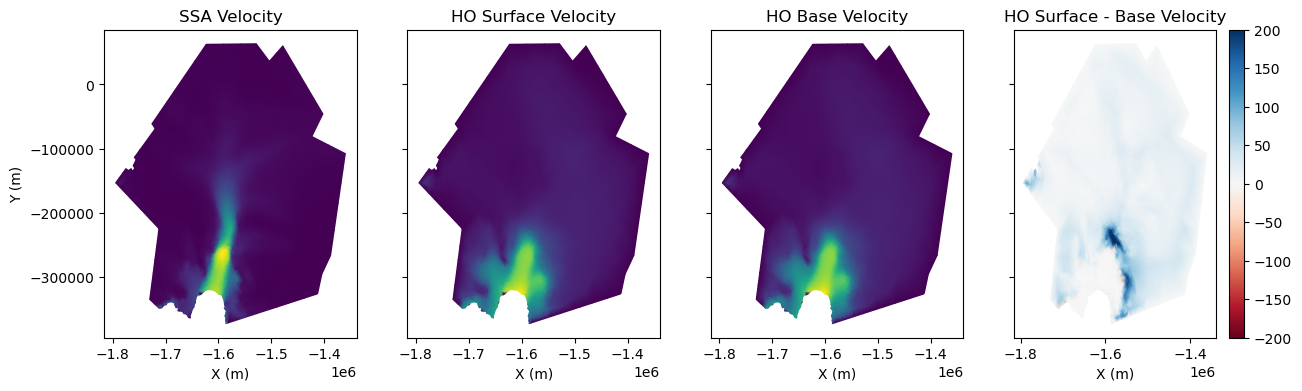
5.1 Plot velocity differences
Now that we have both an SSA and HO solution, we can compare the resultant modelled velocities. Below, we load the HO and SSA models and plot the modelled velocities. For the HO model, we compare the surface and base velocities.
# Load models
md_ho = pyissm.model.io.load_model(tutorial_dir + '/ex2_PIG_HO.nc')
md_ssa = pyissm.model.io.load_model(tutorial_dir + '/ex2_PIG_control_drag.nc')

# Extract relevant velocity fields/layers
ho_surface_vel = md_ho.results.StressbalanceSolution.Vel[md_ho.mesh.vertexonsurface == 1]
ho_base_vel = md_ho.results.StressbalanceSolution.Vel[md_ho.mesh.vertexonbase == 1]
ssa_vel = md_ssa.results.StressbalanceSolution.Vel

# Visualise velocity fields
fig, (ax1, ax2, ax3, ax4) = plt.subplots(1, 4, figsize = (15, 4), sharey = True)
ax1 = pyissm.plot.plot_model_field(md_ssa, ssa_vel, ax = ax1)
ax2 = pyissm.plot.plot_model_field(md_ho, ho_surface_vel, ax = ax2, ylabel = '')
ax3 = pyissm.plot.plot_model_field(md_ho, ho_base_vel, ax = ax3, ylabel = '')
ax4 = pyissm.plot.plot_model_field(md, ho_surface_vel - ho_base_vel, cmap = 'RdBu', show_cbar = True, ax = ax4, vmin = -200, vmax = 200, ylabel = '')

ax1.set_title('SSA Velocity')
ax2.set_title('HO Surface Velocity')
ax3.set_title('HO Base Velocity')
ax4.set_title('HO Surface - Base Velocity')
ℹ️ Processing results group: StressbalanceSolution
ℹ️ Processing results group: StressbalanceSolution
/home/565/lb9857/gitRepos/pyISSM/src/pyissm/model/mesh.py:108: UserWarning: process_mesh: 3D model found. Processing as 2D mesh.
  warnings.warn('process_mesh: 3D model found. Processing as 2D mesh.')
/home/565/lb9857/gitRepos/pyISSM/src/pyissm/model/mesh.py:108: UserWarning: process_mesh: 3D model found. Processing as 2D mesh.
  warnings.warn('process_mesh: 3D model found. Processing as 2D mesh.')
/home/565/lb9857/gitRepos/pyISSM/src/pyissm/model/mesh.py:108: UserWarning: process_mesh: 3D model found. Processing as 2D mesh.
  warnings.warn('process_mesh: 3D model found. Processing as 2D mesh.')
Text(0.5, 1.0, 'HO Surface - Base Velocity')